Diagnostic consistency
Objectives
After successfully completing the workbook students should be able to:
- Describe the meaning of intra- and inter-rater agreement
- Explain why the common use of correlation for measuring agreement is inappropriate
- Identify appropriate techniques for assessing agreement
- Calculate a κ statistic
- Use the Bland-Altman technique to measure agreement
- Interpret the results of an assessment of agreement
Bibliography
Altman, D.G., 1991. Practical Statistics for Medical Research, pp. 397-409. Chapman & Hall, London.
Description of the Bland-Altman method and explanation of how to calculate and use kappa.
Bland, M.J. & D.G. Altman, 1986. Statistical methods for assessing agreement between two methods of clinical measurement. The Lancet 1986 i 307-310.
Explanation of the Bland-Altman method of assessing agreement between continuous variables
Diagnostic consistency
Most clinical measurements are not precise. There are many reasons for this which include:
- It may not be possible to measure something directly - for example, anything which we have to use a radiograph to study
- The measurement may be difficult to make
- The measure may be partially subjective - some plaques score indices are like this, all pain measurement methods are like this
- The patient may vary naturally over time - if we measure a patient's pain, when we are expecting it to vary over a matter of hours it may also fluctuate over a matter of minutes. Thus, there is a random element built into the measurement we actually record.
This may lead us to:
- Check if a measurement method is consistent. Although a consistent measurement is not necessarily accurate we have more faith in it. Also, if a measurement is inaccurate but is consistently inaccurate we can make allowances. (Perhaps we have an old thermometer which always gives a reading 2C higher than the true reading. When using this thermometer we simple subtract 2 from the reading we get.)
- Check if two observers using the same method agree on their results - particularly important when the measurement is partially subjective.
- Check if two methods of measurement agree (perhaps a cheaper method with a more expensive or a quicker with a slower)
The problem we are addressing here is one of measuring agreement, not association. We will illustrate this with two examples, one with a continuous variable and one with a categorical variable.
Continuous variables
Table 1 shows the measurement (in mm) of gum recession by two different dentists for 13 patients.
| Patient | Dentist 1 | Dentist 2 |
|---|---|---|
| 1 | 0·3 | 0·6 |
| 2 | 0·6 | 1·0 |
| 3 | 1·8 | 2·4 |
| 4 | 1·2 | 1·6 |
| 5 | 0·7 | 1·0 |
| 6 | 1·3 | 1·8 |
| 7 | 0·7 | 1·0 |
| 8 | 0·4 | 0·7 |
| 9 | 0·9 | 1·3 |
| 10 | 0·1 | 0·3 |
| 11 | 1·4 | 1·9 |
| 12 | 0·8 | 1·1 |
| 13 | 0·2 | 0·4 |
The data are plotted in figure 1, we can see that they tend to fall on a straight line. If we work out the correlation coefficient we get r = 0·998, the two sets of readings are highly correlated.
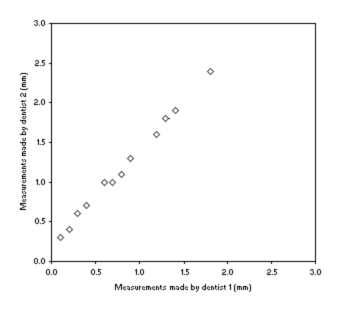
Figure 1: Plot of gum recession measurements made by two dentists
At this point many investigators would stop, they would say there is good agreement because there is good correlation. We, however, are going to do it properly.
The Bland-Altman plot
We are going to use a technique called the Bland-Altman plot. First we fill in the first column of table 2, marked 'Difference' with (Dentist 2) - (Dentist 1) for each patient.
| Patient | Difference | Mean |
|---|---|---|
| 1 | 0·3 | 0·45 |
| 2 | 0·4 | 0·80 |
| 3 | 0·6 | 2·10 |
| 4 | 0·4 | 1·40 |
| 5 | 0·3 | 0·85 |
| 6 | 0·5 | 1·55 |
| 7 | 0·3 | 0·85 |
| 8 | 0·3 | 0·55 |
| 9 | 0·4 | 1·10 |
| 10 | 0·2 | 0·20 |
| 11 | 0·5 | 1·65 |
| 12 | 0·3 | 0·95 |
| 13 | 0·2 | 0·30 |
Notice that Dentist 2 consistently gives higher readings than Dentist 1. So, it is perfectly possible for two observers to disagree about measurements yet have their measurement correlate.
Now we fill in the 'Mean' column with the mean of the two readings for each patient. We can now plot 'Mean' against 'Difference' and get figure 2, below.
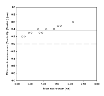
Figure 2: Scatterplot of gum recession measurements made by two dentists
If the measurements all agreed perfectly they would all fall on the dashed line at '0' difference. The fact that they all fall above this line indicates to us that there is a disagreement.
The solid line on the plot tells us something more about the disagreement. If you work out the mean of the differences (i.e. all 13 difference added together and divided by 13) then you will see that the solid horizontal line is plotted at this value.
This 'mean difference' is an estimate of the bias between the two dentists. If the mean difference is small then the bias is small, there is good agreement on average. If the mean difference is large then there is poor agreement, one method is biased relative to the other. There is not a statistical test to tell us whether the bias we have calculated is good or not. You have to use your clinical judgement to decide whether or not the bias (0·36 in this case) is acceptable or not. We would also have to decide if was acceptable that Dentist 2 alwaysy gave higher values than Dentist 1.
Remember: correlation is a measure of association not a measure of agreement. It is wrong to use correlation as a measure of agreement.
| Patient | Dentist A | Dentist B | Difference | Mean |
|---|---|---|---|---|
| 1 | 0·3 | 0·1 | -0·2 | 0·20 |
| 2 | 0·6 | 0·0 | -0·6 | 0·30 |
| 3 | 1·8 | 0·3 | -1·5 | 1·05 |
| 4 | 1·2 | 0·5 | -0·7 | 0·85 |
| 5 | 0·7 | 3·3 | 2·6 | 2·00 |
| 6 | 1·3 | 0·6 | -0·7 | 0·95 |
| 7 | 0·7 | 0·3 | -0·4 | 0·50 |
| 8 | 0·4 | 1·3 | 0·9 | 0·85 |
| 9 | 0·9 | 0·6 | -0·3 | 0·75 |
| 10 | 0·1 | 0·4 | 0·3 | 0·25 |
| 11 | 1·4 | 1·1 | -0·3 | 1·25 |
| 12 | 0·8 | 2·1 | 1·3 | 1·45 |
| 13 | 0·2 | 1·4 | 1·2 | 0·80 |
Table 3 shows the measurement (in mm) of gum recession by two different dentists for 13 patients. The mean of the differences is 0·12mm, indicating that on average the agreement between the dentists is quite good. This is also seen in figure 3: the line indicating the bias is close to zero.
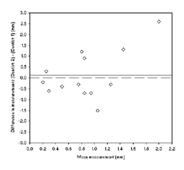
Figure 3: Scatterplot of gum recession measurements made by dentists A and B
However, it is possible for two observers to agree very well on average but be unlikely to give good agreement for a particular individual. If a situation like that in table 4 occurred we would have a mean difference of zero. That is, the bias is zero, on average the dentists agree, yet we can see from the table that they actually disagree a lot for any individual patient. We need a measure that can describe this variation in agreement for individual patients.
| Patient | Dentist X | Dentist Y | Difference | Mean |
|---|---|---|---|---|
| 1 | 0·7 | 0·1 | -0·6 | 0·40 |
| 2 | 0·1 | 0·7 | 0·6 | 0·40 |
| 3 | 1·5 | 0·3 | -1·2 | 0·90 |
| 4 | 0·6 | 1·8 | 1·2 | 1·20 |
If we work on the assumption that the differences would be reasonably symmetric (i.e. we are as likely to get differences greater than the bias as differences smaller than the bias) we would expect that about 95% of differences to fall within the range:
(mean of differences) ± 2x(standard deviation of differences)
These are called the 95% limits of agreement.
The standard deviation of the differences in table 3 is 1·10, the mean difference is 0·12.
(mean of differences) - 2x(standard deviation of differences) = -2.08
(mean of differences) + 2x(standard deviation of differences) = 2.33
We now draw two more (horizontal) lines onto figure 3 at these values. This is now a complete Bland-Altman plot, figure 4. We now have both a pictorial and a numeric description of the 95% limits of agreement. Once again there is no statistical way to judge if these are acceptable. You have to decide if it is clinically acceptable for 95% of the measurements to disagree by no more than these amounts.
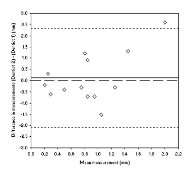
Figure 4: Bland-Altman plot of gum recession measurements made by dentists A and B
The standard deviation of the differences for table 1 is 0·12. Using this information we can draw the 95% limits of agreement onto figure 1 and get figure 5.
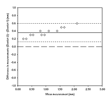
Figure 5: Bland-Altman plot of gum recession measurements made by dentists 1 and 2
So, what is the additional information we get from the Bland-Altman plot compared to just calculating the bias and 95% limits of agreement numerically?
Well, inspection of the plot can tell us if there variation in agreement across the range of measurements. If we look at figure 5 we can see that not only are measurements biased but that the disagreement increases as the measurements get higher. Our final piece of interpretation of this data set might be to note that the 95% limits of agreement do not include zero so thes two dentists are very unlikely to ever agree on a measurement. Examining figure 4, there is a small bias but the 95% limits of agreement are unacceptably wide. We might note that there is some evidence for the disagreement to larger as the measurements get larger.
Categorical variables
χ2 test
The χ2 test measures association not agreement.
Just as correlation is not used to measure agreement for continuous variables the χ2 test is not used to measure agreement for categorical variables.
Kappa, κ
[κ is a Greek letter, pronounced kappa.]
To compare the agreement between different observers we use the kappa statistic. For example, if two dentists assess the level of gum disease in 50 patients and diagnose them as having a clinical or a sub-clinical level of disease as follows:
| Dentist 2 | ||||
| Clinical | Sub-clinical | Total | ||
| Dentist 1 | Clinical | 12 | 3 | 15 |
| Sub-clinical | 4 | 31 | 35 | |
| Total | 16 | 34 | 50 | |
A common error in analysing agreement with this sort of data is to calculate the proportion, or percentage, agreement. Here, out of 50 measurements 12 + 31 = 43 agreed. This gives us a 86% agreement.
There is a problem with this: no account taken of chance agreement. We would expect some measurements to agree just by chance even if the two dentists were making their diagnoses randomly. So any measure of agreement has to take this into account.
So, first we need to assess the level of agreement we would expect by chance. As with the χ2 test we can calculate the expected frequencies of each cell by the formula:
Expected frequency = (row total) x (column total) ÷ (overall total)
For the table above this gives us:
| Dentist 2 | ||||
| Clinical | Sub-clinical | Total | ||
| Dentist 1 | Clinical | 4·8 | 10·2 | 15 |
| Sub-clinical | 11·2 | 23·8 | 35 | |
| Total | 16 | 34 | 50 | |
The expected number of agreements is obtained by adding together the 'Clinical/Clinical' cell and the 'Sub-clinical/Sub-clinical' cell. For this table the expected number of agreements is:
28·6
We can express this as a proportion by dividing this by 50, the total number of measurements. For this table the expected proportion of agreement is:
28·6 ÷ 50 = 0·572
Our question is now "how much better was the observed proportion of agreement than the expected proportion of agreement?"
The observed proportion of agreement was: 43 ÷ 50 = 0·860
The maximum possible proportion of agreement is 1·00.
We express the observers' agreement as a proportion of the possible scope for doing better than chance, this is kappa:
![]()
In this case:
κ = (0·860 - 0·572) ÷ (1 - 0·572) = 0·67
In general κ > 0·6 is regarded as good agreement. The table below is a guide to assessing how strong an agreement is, based on κ.
| Value of κ | Strength of agreement |
|---|---|
| <0·21 | Poor |
| 0·21 - 0·40 | Fair |
| 0·41 - 0·60 | Moderate |
| 0·61 - 0·80 | Good |
| 0·81 - 1·00 | Very good |
Confidence intervals can be calculated for κ although this step is frequently missed out. The procedure is given in Altman (p. 405).
What if there are more than two categories for the variable?
κ can also be calculated for larger (square) contingency tables.
Weighted κ
If the categories are ordered a weighted version of kappa can be calculated in these circumstances to take into account the level of disagreement.
| Observer 2 | |||||
| 1 | 2 | 3 | Total | ||
| Observer 1 | 1 | 85 | 9 | 6 | 100 |
| 2 | 12 | 60 | 28 | 100 | |
| 3 | 3 | 31 | 66 | 100 | |
| Total | 100 | 100 | 100 | 300 | |
In the above table the cells containing '3' and '6' would be accorded more importance (weight) when calculating κ than those containing '12', '31', '9', and '28' because they represent a greater level of disagreement (2 categories difference rather than 1). The procedure for calculating weighted κ is give in Altman (p. 407), but you don't need to learn it.