Non-parametric tests
Objectives
At the end of the lecture students should be able to:
- Understand why we use non-parametric tests
- Make a decision as to the appropriate univariate tests for simple data sets
Bibliography
All the recommended course books will cover most of the material here in various amounts of complexity and detail
Introduction
We use non-parametric tests when we do not expect our data to conform to a parametric distribution such as the normal distribution or the t distribution.
They can also be used if other assumptions about the data needed for certain tests are violated. (E.g. equality of standard deviations for the two-sample t test.
The most common non-parametric tests we shall come across are the Wilcoxon test for paired data (more properly the Wilcoxon matched pairs signed rank sum test) and the Mann-Whitney U test (sometimes called the Mann-Whitney-Wilcoxon test, the Wilcoxon T test, the Wilcoxon two-sample test, or the Wilcoxon W test) for unpaired data. These tests are based on ranking the data and looking at the ranks rather than the actual values of the observations.
There is confusion over the naming of these tests in the literature. Indeed, some computer programs will do things like performing a Mann-Whitney test but express the result in terms of Wilcoxon's W.
Non-parametric tests are applicable in a wider range of situations but the are, in general, less powerful: they cannot detect differences as small as the ones detectable by the equivalent parametric tests.
The phrase non-parametric does not mean we necessarily make no assumptions about the data. For example the Wilcoxon matched pairs signed rank sum test makes the assumption that the populations the samples come from are symmetric.
Example: The Mann-Whitney test
The following table shows the clinical attachment level of two groups of patients (smokers and non-smokers) at the end of a period of periodontological treatment. We want to know if there is a difference between the groups.
| Non-smoker | CAL (mm) | Smoker | CAL (mm) | |
|---|---|---|---|---|
| 1 | 1·0 | 14 | 2·8 | |
| 2 | 0·6 | 15 | 0·0 | |
| 3 | 1·1 | 16 | 4·2 | |
| 4 | 1·2 | 17 | 1·3 | |
| 5 | 0·7 | 18 | 3·6 | |
| 6 | 1·3 | 19 | 1·6 | |
| 7 | 0·9 | 20 | 0·9 | |
| 8 | 0·4 | 21 | 1·3 | |
| 9 | 0·9 | 22 | 1·0 | |
| 10 | 0·2 | 23 | 1·5 | |
| 11 | 1·4 | 24 | 2·8 | |
| 12 | 0·9 | 25 | 2·8 | |
| 13 | 0·8 | 26 | 2·0 |
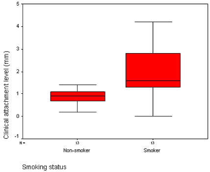
Examination of the data using a box and whisker plot leads us to believe that the data may not be normally distributed. It would therefore be unwise to use a t test. We need to use a Mann-Whitney test.

The Mann-Whitney test calls for the observations of two groups to be ranked as if they were from a single population. The null hypothesis of the test is that the two samples are drawn from identical populations: there is no difference between the two populations the samples are drawn from. So, first we order the data, taking no account of which group the data is from:
![]()
If there are ties in the data (marked in bold above) we have to adjust the ranks. Observations with the same value are given the mean rank of all observations with that value. So the four observations with value 0·9 which were ranked 7, 8, 9 and 10 have their ranks changed to (7+8+9+10)÷4 = 8·5. Other ties are treated similarly:
![]()
We then look at the sums of the ranks of the data for the two groups:
![]()
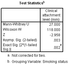
We see that the rank sum for smokers is 233 and for non-smokers it is 118. Under the null hypothesis of no difference we would expect both rank sums to be equal (175·5 in this case), give or take some random variation. You do not need to know how to calculate if the difference in rank-sums we observe is significantly different from no difference, SPSS (or any similar statistical package) can do this:


Mann-Whitney U and Wilcoxon W are two alternative statistics that are used to determine if the difference in ranks ar significant (like the t in a t test). Z is the conversion of these two statistics to a Z score (a clever bit of mathematical trickery that makes it easier to arrive at a P value). The P value we want is labelled Asyp. Sig. (2-tailed). The other option has a note by it saying that it is not corected for ties. We always want the version that is corrected for ties. We have P = 0·002, a statistically significant result for α = 0·05, we can safely reject the null hypothesis of no difference.
When presenting the results of a Mann-Whitney test ensure that you quote the sample sizes and the P value (the citing of the value of U is optional. It is also important to give something extra to aid clinical interpretation, such as the box plot above or the medians and IQRs of the two groups.
Notes:
- If there are a lot of tied ranks then adjustments need to be made to the test statistic. Check your program does this
- Care needs to be taken when using computer programs that you are using the right test - names can be confusing
- We should have group sizes of ten or more for the approximations of the Mann-Whitney test to be valid
Which test to use

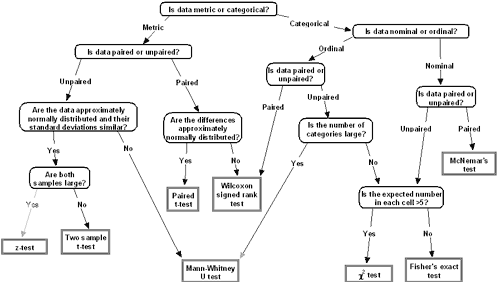
The flowchart above should guide you to the correct test to use for a variety of data sets.
Notes:
- I would recommend never using the z test, the t test is perfectly OK in the situations the flowchart recommends a z test. (This avoids having to decide what is large!)
- There is some argument about whether a Mann-Whitney test is really suitable for categorical ordinal data with large numbers of categories. It's probably better to seek advice if you think you might want to do this.