Inference and P values
Objectives
At the end of the lecture and having completed the exercises students should be able to:
- Understand the principles of hypothesis-testing and be able to interpret P values correctly
- Carry out a t test
Hypothesis testing and estimation
Hypothesis testing and estimation are two alternative approaches to statistical inference. We looked at estimation in the last lecture. In general most medical statisticians would prefer estimation to hypothesis testing, if they were forced to make a choice. Hypothesis testing, however, is still an important tool, although probably somewhat overused. It was overwhelming the preferred approach until fairly recently.
The problem
A previous MDentSci student was looking at the effects of various chocolates on pH of saliva. She wanted to see if the minimum salival pH produced by two different chocolates was different. After measuring the pH of fourteen subject who had eaten the two chocolates she got the following results:
| Sample size | Mean minimum pH | Std. deviation of minimum pH | |
|---|---|---|---|
| Chocolate A | 14 | 5·86 | 0·39 |
| Chocolate B | 14 | 5·53 | 0·31 |
She observed a difference between the mean values for the minimum pH but she wanted to know if this difference could have arisen by chance. A hypothesis test is required.
Structure of a hypothesis test
The following is the basic structure of a hypothesis test:
1) State the null and alternate hypotheses
The null hypothesis is usually of the form: there is no difference between the two groups. Or: our new treatment would have no effect.
Which means that the alternate hypothesis would be: there is a difference. Or: our new treatment has an effect.
- Note that our alternate hypothesis does not state what the difference is (or even which direction it is in)
- We always test the null hypothesis
In our case the null hypothesis is "There is no difference in the minimum salival pH produced by chocolates A and B".
In a hypothesis test we calculate a probability called the P value.
The P value is defined as the probability of obtaining the result, or a more extreme result, if the null hypothesis is true.
2) Decide a level of significance (α)
We need to decide what level of probability we will accept as being 'unlikely'. Conventionally a 5% probability is considered sufficiently unlikely. We tend to choose:
α = 0·05
3) Define and evaluate a test statistic
- We choose a test statistic which has a distribution which matches our data
- There are many of these that we will come across such as t, &chi2 and Mann-Whitney U
We shall be using a statistic known as t (or sometimes Student's t, after the person who discovered it). t is a statistic that is appropriate for examining the means of samples drawn from a normal distribution.
Although we learned in the previous unit that the distribution of means of samples from a normal population is itself normal, this is not quite the case for small samples. Small samples tend to follow a t distribution.
What is small?
Traditionally <30 has been regarded as small. In practice we can regard all samples as 'small' as a way of ensuring we do not make mistakes
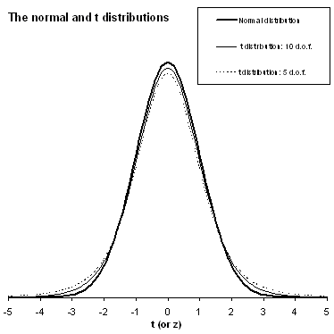
t distributions
- There are many different t distributions one for each number of degrees of freedom
- Degrees of freedom are related to sample size in a particular way for each type of t test
- The greater the degrees of freedom the more closely the t distribution resembles the normal distribution
We want to compare the means of two samples of pH data, we shall be using the two-sample t test (more often just referred to as the t test).
In this case t is defined as:
![]()
(The difference in means divided by the standard error of the difference)
The standard error of the difference is calculated by using the formula:
![]()
Where s is the pooled standard deviation. This is calculated as so:
![]()
(n1 and n2 are the sizes of the two samples and s1 and s2 are their standard deviations)
You do not need to remember these formulae.
Using the values from the study we get a pooled standard deviation of 0·352 Which gives a standard error of 0·133 This gives us t = 2·478
4) Calculate the P value
Essentially what we are doing is seeing where on the appropriate t distribution our calculated value of t lies - how unlikely is our value of t if the null hypothesis were true. (0≤P≤1)
Which t distribution do we use?
We need to calculate the degrees of freedom. For a two sample t test the degrees of freedom is given by:
d.o.f = n1 + n2 - 2
So in our case we have 26 degrees of freedom.
If we were using a computer we could get an exact P value for the hypothesis test. Doing it by hand we have to look up a set of critical values for our t distribution. For 26 degrees of freedom the table looks like this:
| Two-tailed probability (P) | |||||
|---|---|---|---|---|---|
| Degrees of freedom | 0·1 | 0·05 | 0·02 | 0·01 | 0·001 |
| 26 | 1·706 | 2·056 | 2·479 | 2·779 | 3·707 |
If our calculated value of t if greater than a critical value then the P value is less than the value at the top of the column. Our value of t is 2·478, this is smaller than 2·479 so the P value for our study is more than 0·02:
P>0·02
Putting these together we get:
0·05>P>0·02
(If we had done this by computer we would have got the result: P = 0·04)
5) Interpret the results
Since our P value is less than our preset value of α (0·05) then we have a statistically significant result.
There is a statistically significant difference of 0·33 between the mean minimum pH produced by the two chocolates.
Or we might comment that there is strong evidence against the null hypothesis of no difference between the two chocolates' effects on salivary pH.
Points to note
- P values should be given to no more than three decimal places (two is normally sufficient)
- P values less than 0·001 should normally be expressed as P<·001 rather than giving the exact value
- Always give the difference observed as well as the test results
- Always state which test you have used and what value of α you chose
What difference would estimation have made?
Although we now have strong evidence against the null hypothesis it is couched in statistical terms, there is a statistically significant difference. Clinical interpretation is possible but would be made easier if we could put a 95% confidence interval on the difference between the means.
We do this in much the same way as we learned in the previous unit but make one adjustment for greater accuracy.
Previously we defined the 95% confidence interval as:
sample mean - 1·96 standard errors to sample mean + 1·96 standard errors
Strictly speaking this is only true for large sample sizes, for small sample sizes we use:
sample mean - t standard errors to sample mean + t standard errors
Where t is the critical value for P = 0·05 for the appropriate number of degrees of freedom
As we are looking at the difference between two means then we want the 95% confidence interval for this difference:
difference in means - t standard errors to difference in means + t standard errors
Difference in means is: 0·33
Standard error of difference in means: 0·133
t = 2·056
This gives us a 95% confidence interval for the difference in means:
From 0·06 to 0·60
We can now make a better clinical interpretation. As the true difference in means could plausibly be as low as 0·06 then we would probably feel that the clinical significance of the difference is low.
Note that we can also use the confidence interval to assess statistical significance. If the 95% confidence interval includes 0 then there could plausibly be no difference, so we have a statistically significant result.
Difference between P values and confidence intervals
- A P value measures the strength of evidence against the null hypothesis.
- A P value is the probability of getting a result as, or more, extreme if the null hypothesis were true.
- It is easy to compare results across studies using P values
- P values are measures of statistical significance
- Confidence intervals give a plausible range of values in clinically interpretable units
- Confidence intervals enable easy assessment of clinical significance
Presenting the results
The difference in mean minimum salivary pH observed between two samples of fourteen individuals was 0·33 (95% CI from 0·06 to 0·60), a two-sample t test (26 d.o.f.) gave a P value of 0·04. Whilst we observed a statistically significant difference between the effects of the two chocolates we feel that there is unlikely to be any clinical significance to the difference which could plausibly be as low as 0·06.
Note
We do not use a dash instead of the word "to". ("95% CI from 0·06 - 0·60" is not encouraged.) This is to avoid potential confusion with negative numbers.
Final note
If we had looked at the differences the other way round (B - A rather than A - B) we would have got a negative value for t. This is not a problem. It would have been the same value, but negative (-2·478). We could look it up in the table by simply ignoring the minus sign. (We are taking advantage of the fact the t distribution is symmetric.)